Kaplan Meier Survival Curves

---

Introduction to Kaplan-Meier Method

From the pervious chapter, we learned that the data layout that we typically use for survival analysis is given by the table shown here:

Ordered failure times $(t_{(f)})$	# of failures $(m_f)$	# censored in $[t_{(f)},t_{(f-1)}) (q_f)$	Risk set R $(t_{(f)})$
$t_{(0)} = 0$	$m_0=0$	$q_0$	$R(t_{(0)})$
$t_{(1)}$	$m_1$	$q_1$	$R(t_{(1)})$
$t_{(2)}$	$m_2$	$q_2$	$R(t_{(2)})$
.	.	.	.
.	.	.	.
.	.	.	.
$t_{(k)}$	$m_k$	$q_k$	$R(t_{(k)})$

This layout is the basis upon which Kaplan-Meier survival curves are derived. The first column represents ordered survival times from smallest to largest. The second column represents frequency counts for failures at each distinct failure time. The third one represents frequency counts of those persons censored in the time interval from failure time $t_{(f)}$ up to but not including the next failure time $t_{(f+1)}$. The last column gives the risk set, which denotes the collection of individuals who have survived at least to time $t_{(f)}$.

An Example of Kaplan-Meier Curves

Let's still take a look at the dataset from the last chapter:

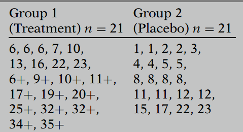
We list these data as the KM table:

Group 1	Group 2

Each table begins with a survival time of zero, even though no subject actually failed at the start of follow-up. The reason for the zero is to allow for the possibility that some subjects might have been censored before the earliest failure time.

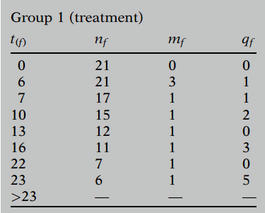
We also have each table contain a column denoted as $n_f$ that gives the number of subjects in the risk set at the start of the interval. $n_f$ counts subjects at risk for failing instantaneously prior to time $t_{(f)}$.

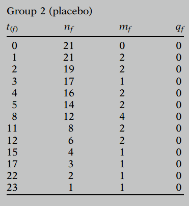
Now let's talk about how to compute the KM curve for group 2.

For group 2, because we don't have any censored subjects, the computation of the KM curve is straightforward.

$t_{(f)}$	$n_f$	$m_f$	$q_f$	$\hat S(t_{(f)})$
0	21	0	0	1
1	21	2	0	19/21=0.90
2	19	2	0	17/21=0.81
3	17	1	0	16/21=0.76
4	16	2	0	14/21=0.67
5	14	2	0	12/21=0.57
8	12	4	0	8/21=0.38
11	8	2	0	6/21=0.29
12	6	2	0	4/21=0.19
15	4	1	0	3/21=0.14
17	3	1	0	2/21=0.10
22	2	1	0	1/21=0.05
23	1	1	0	0/21=0.00

Here, $\hat S(t_{(f)})$ is the survival probability at time $t_{(f)}$. The probability of surviving past the first ordered failure time of $1$ week is given by $19/21$ or $0.90$ because $2$ people failed at $1$ week, so that $19$ people from the original $21$ remain as survivors past $1$ week. Similarly, the next probability concerns subjects surviving past $2$ weeks, which is $17/21$ or $0.81$ because $2$ subjects failed at $1$ week and $2$ subjects failed at $2$ weeks leaving $17$ out of the original $21$ subjects surviving past $2$ weeks.

Recall that no subject in group 2 was censored, so the $q$ column for group 2 consists entirely of zeros. If some of the q's had been nonzero, an alternative formula for computing survival probabilities would be needed. This alternative formula is called the Kaplan-Meier (KM) approach and can be illustrated using the group 2 data even though all values of $q$ are zero.

For instance, an alternative way to calculate the survival probability of exceeding $4$ weeks for the group 2 data can be written using the KM formula shown here. This formula involves the product of conditional probability terms. That is, each term in the product is the probability of exceeding a specific ordered failure time $t_{(f)}$ given that a subject survives up to that failure time. We have:

$$\hat{S}(4)=1\cdot\frac{19}{21}\cdot\frac{17}{19}\cdot\frac{16}{17}\cdot\frac{14}{16}=\frac{14}{21}=0.67$$

Thus, in the KM formula for survival past $4$ weeks, the term $19/21$ gives the probability of surviving past the first ordered failure time, $1$ week, given survival up to the first week. Note that all $21$ persons in group 2 survived up to $1$ week, but that $2$ failed at $1$ week, leaving $19$ persons surviving past $1$ week.

Similarly, the term $16/17$ gives the probability of surviving past the third ordered failure time at week $3$, given survival up to week $3$. There were $17$ persons who survived up to week $3$ and $1$ of these then failed, leaving $16$ survivors past week $3$. Note that the $17$ persons in the denominator represents the number in the risk set at week $3$.

Notice that the product terms in the KM formula for surviving past $4$ weeks stop at the 4th week with the component $14/16$. Similarly, the KM formula for surviving past $8$ weeks stops at the eighth week:

$$\hat{S}(8)=1\cdot\frac{19}{21}\cdot\frac{17}{19}\cdot\frac{16}{17}\cdot\frac{14}{16}\cdot\frac{12}{14}\cdot\frac{8}{12}=\frac{8}{21}=0.38$$

Generally speaking, KM formula for a survival probability is limited to product terms up to the survival week being specified. Thus, KM formula is often called "product-limit" formula.

Now let's consider the KM formula for group 1 data.

$t_{(f)}$	$n_f$	$m_f$	$q_f$	$\hat S(t_{(f)})$
0	21	0	0	$1$
6	21	3	1	$1\times\frac{18}{21}=0.8571$
7	17	1	1	$0.8571\times\frac{16}{17}=0.8067$
10	15	1	2	$0.8067\times\frac{14}{15}=0.7529$
13	12	1	0	$0.7529\times\frac{11}{12}=0.6902$
16	11	1	3	$0.6902\times\frac{10}{11}=0.6275$
22	7	4	0	$0.6275\times\frac{6}{7}=0.5378$
23	6	2	5	$0.5378\times\frac{5}{6}=0.4482$

The other survival estimatesb are calculated by multiplying the estimate for the immediately preceding failure time by a fraction. For example, the fraction is $18/21$ for surviving past week $6$, because $21$ subjects remain up to week $6$ and $3$ of these subjects fail to survive past week $6$. The fraction is $16/17$ for surviving past week $7$, because $17$ people remain up to week $7$ and $1$ of these fails to survive past week $7$. The other fractions are calculated similarly.

Plots of the KM curves for groups 1 and 2 are shown here on the same graph. Notice that the KM curve for group 1 is consistently higher than the KM curve for group 2. These figures indicate that group 1, which is the treatment group, has better survival prognosis than group 2, the placebo group.

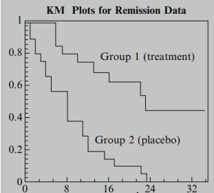
Note that we can obtain KM plots from R using the "survival" package.

---

General Features of KM Curves

General KM Formula

$$\begin{aligned} \hat{S}\left(t_{(f)}\right)= & \prod_{i=1}^f \hat{P} r\left[T>t_{(i)} \mid T \geq t_{(i)}\right] \\ = & \hat{S}\left(t_{(f-1)}\right) \times \hat{\operatorname{P}}\left(T>t_{(f)} \mid T \geq t_{(f)}\right) \end{aligned}$$

For example, the probability of surviving past $10$ weeks is given in the table for group 1 by $.8067$ times $14/15$, which equals $.7529$. But the $.8067$ can be alternatively written as the product of the fractions $18/21$ and $16/17$. Thus, the product limit formula for surviving past $10$ weeks is given by the triple product shown here.

$$\begin{aligned} \hat{S}(10) & =.8067 \times \frac{14}{15}=.7529 \\ & =\frac{18}{21} \times \frac{16}{17} \times \frac{14}{15} \end{aligned}$$